Disclaimer: This contains a 75-minute lesson plan that I developed for ESCI 4701 (Geomorphology) during the Fall semester of 2022 at the University of Minnesota. The lesson plan includes animations rendered using Blender as well as an interactive landscape evolution model (Javascript) that students can use to explore qualitative relationships. Also included is an additional 75-minute activity where students use a Python-notebook (written in Google Collab) to explore landscape evolution using the Landlab library.

Learning Goals

1. Review the main components of landscape evolution models
2. Understand basic concepts for running numerical models
3. Determine how geomorphic processes interact with interactive models
4. Introduce the concept of dynamic equilibrium in landscape evolution models

Landscape Evolution Model Components

Landscape evolution models simulate how the surface of the Earth changes over time. The location of the Earth’s surface is referred to as elevation, signified here as $\eta$. In this notation, the change in elevation with time, $t$ is given by:

\begin{align} \tag{1} \frac{\partial \eta}{\partial t} \end{align}

In LEMs, we study how landscapes change according to three processes: Tectonic, Hillslope, and Fluvial. Before we build a full LEM, let’s explore each process individually.

Tectonic Processes

Tectonic processes introduce material into the landscape through rock uplift. The most standard approach assumes that the rate of rock uplift, $U$, is both steady and uniform. $U$ determines the rate at which the landscape rises [Eqn. 2].

\begin{align} \tag{2} \frac{\partial \eta}{\partial t} = U \end{align}

Fig. 1: Landscape subjected to tectonic uplift only. $U$ = 1 mm⁄yr. At the end of the video, landscape is uplifted 500 m. Vertical exaggeration = 2.0; 1 sec = 50 kyr.

Fluvial Processes

Fluvial erosion processes in landscape evolution models are simulated using the stream power incision model [Eqn. 3] (a.k.a. stream power law).

\begin{align} \tag{3} \frac{\partial \eta}{\partial t} = - KA^mS^n \end{align}

Fig. 2: Channel profile view of knickpoint retreat driven by fluvial erosion. Increasing the value of $K$ increases the rate of knickpoint retreat. Drain-age area, $A$, and $U$ are constant in these simulations.

An important parameter is $K$, which determines how erodible rock is to flow. It contains information about:

• lithology
• climate
• gravity
• fluid density

$K$ controls:

• the rate of erosion for a given drainage area and slope
• the rate of knickpoint retreat [Fig. 2]
• the slope of the channel at equilibrium

Fig. 3: Previously uplifted landscape subjected to fluvial erosion only. $K$ = 0.00001 yr^-1, and the total basin area is 200 km² (20 km x 10 km). The left boundary is open (outlet) and all other boundaries are closed (walls). Vertical exaggeration = 2.0; 1 sec = 50 kyr.

Hillslope Processes

Hillslope processes in landscape evolution models are simulated using a hillslope diffusion model [Eqn. 4].

\begin{align} \tag{4} \frac{\partial \eta}{\partial t} = D\nabla^2\eta \end{align}

Fig. 4: 1D profile view of hillslope diffusion using different values of $D$.

$D$ determines the rate of hillslope diffusion [Fig. 4]. It models soil movement via:

• rainsplash
• bioturbation
• freeze-thaw processes
• creep
• agricultural tillage

What is $\nabla^2\eta$? It is a symbol that represents the sum of second derivatives in the x and y direction, i.e., $\nabla^2\eta = \left(\frac{\partial^2\eta}{\partial x^2}\right) + \left(\frac{\partial^2\eta}{\partial y^2}\right)$. Remember from your calculus class that the 2nd derivative represents the slope of slope? We call $\nabla^2\eta$, topographic curvature.

Fig. 5: Previously uplifted and fluvial eroded landscape subjected to hilllslope processes only. $D$ = 0.2 m²⁄yr. A relatively high $D$ value is used for illustration. Vertical exaggeration = 2.0; 1 sec = 50 kyr.

Variables and Parameter Definitions

Parameter	Fundamental Unit	Description
$\eta$	L	Elevation
$t$	T	Time
$U$	LT$^{-1}$	Uplift Rate
$K$	L$^{(1-2m)}$T$^{-1}$	Erodibility
$A$	L$^2$	Drainage Area
$S$	-	Channel Slope
$m$	-	Area Exponent
$n$	-	Slope Exponent
$D$	L$^2$T$^{-1}$	Diffusion Coefficient
$\nabla^2\eta$	L$^{-1}$	Topographic Curvature

Building a Numerical Model

In order to model the evolution of landscapes, we must specify the landscape’s starting point, named an initial condition. You may have noticed in the movies above that our landscape has defined borders. We must also define rules of how the landscape behaves at these borders, named boundary conditions.

• Initial Conditions Types
  • slanted topography
  • randomized topography
  • endless options…
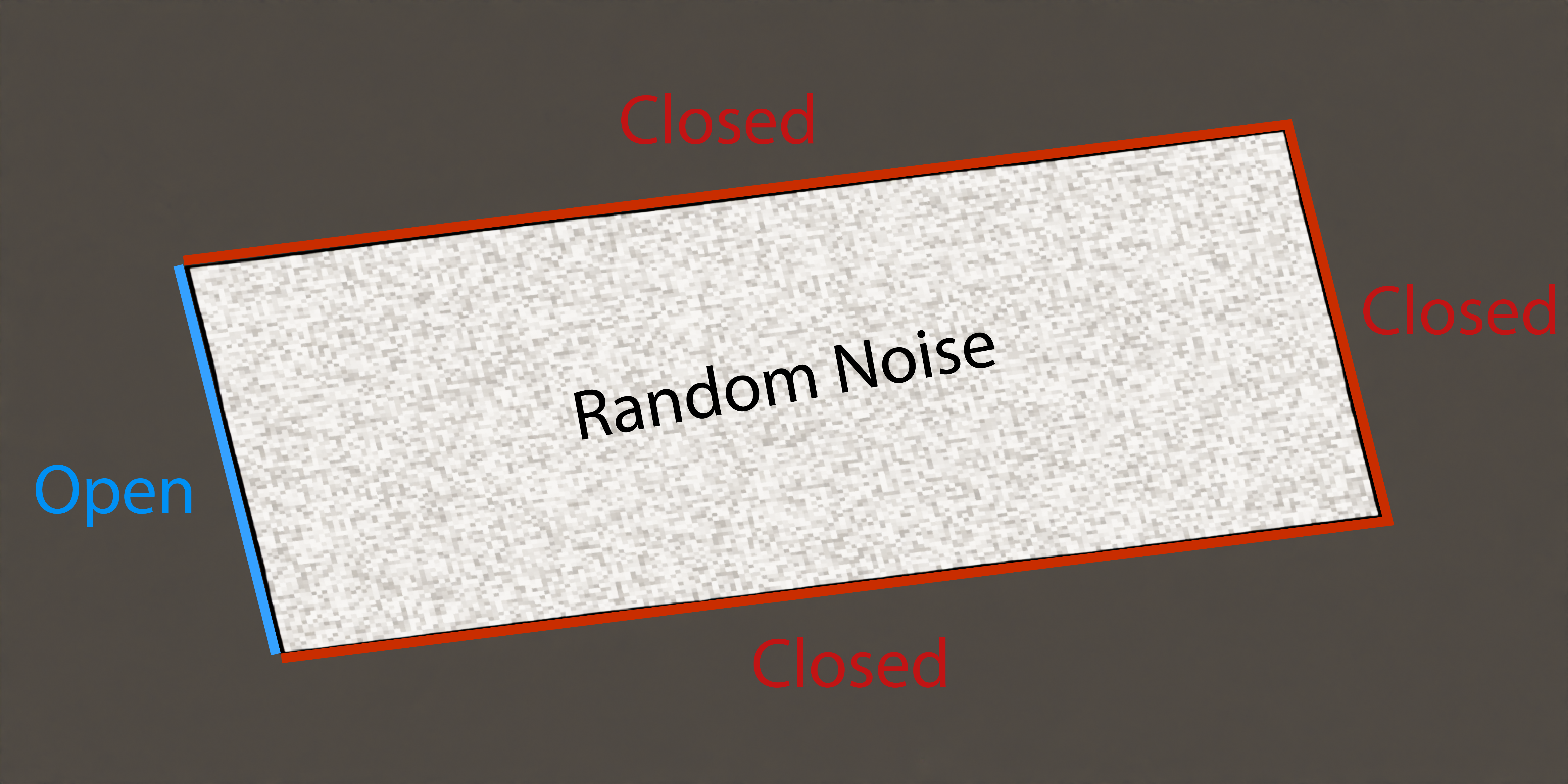
• Boundary Conditions Types
  • open - water/sediment can travel through boundary<
  • closed- water/sediment cannot travel through boundary
  • fixed value - elevation is fixed to a specified value
  • fixed gradient - elevation gradient is fixed to a specified value
  • periodic - water/sediment that leaves one side comes out the other side

Fig. 6: The initial conditions and boundary conditions used in this presentation. The initial condition is a horizontal plane with added randomized perturbations. The boundary conditions are open (blue) and closed (red).

All Together Now!

We now know the three main components of landscape evolution models and some basic concepts for running numerical models. It is time to put it all together [Eqn. 2, Eqn. 3, and Eqn. 4] and run the numerical model. Here is the full conservation equation [Eqn. 5].

\begin{align} \tag{5} \frac{\partial \eta}{\partial t} = U - KA^mS^n + D\nabla^2\eta \end{align}

Things to ponder…

1. Describe the two stages of the numerical simulation.
2. What happens to the landscape after the 10 second mark?
3. Where do you think Eqn. 3 is most important, what about Eqn. 4? Why?

Fig. 7: Landscape evolution incorporating all the processes. $U$ = 1 mm⁄yr; $K$ = 0.00001 yr^-1; $D$ = 0.1 m²⁄yr. Vertical exaggeration = 2.0; 1 sec = 120 kyr.

Dynamic Equilibrium

Around the 10 second mark, the landscape reaches an steady state, which we call dynamic equilibrium. In this state, elevation no longer changes, which can represented by

\begin{align} \tag{6} \frac{\partial \eta}{\partial t} = 0 \end{align}

Inserting Eqn. 6 into Eqn. 5 yields the following:

\begin{align} \tag{7} U = KA^mS^n - D\nabla^2\eta \end{align}

When the landscape reaches dynamic equilibrium, it configures itself, so the sum of fluvial and hillslope processes equal the uplift rate.

No Uplift

Setting $U$ to zero means that

\begin{align} \tag{8} KA^mS^n = D\nabla^2\eta \end{align}

A non-zero solution would mean the landscape only contains concave-upward hillslopes. This is not a stable condition because it is difficult to create a landscape without concave-downward regions (ridges). Instead, a landscape without uplift would tend towards a solution where both slope and curvature are zero (a flat horizontal plane).

Discussion Questions

1. Do landscapes that have been tectonically inactive for long periods become flat in nature?
2. Why or why not?

River Dominated

In rivers, where hillslope processes can be ignored, the Eqn. 7 simplifies to

\begin{align} \tag{9} U = KA^mS^n \end{align}

• For a constant $A$, $S \propto \frac{U}{K}^{1/n}$
• For a constant $U$ and $K$, $A \propto S^{-m/n}$

Discussion Questions

1. What do these proportional statements tell us how the landscape responds to $U$ and $K$?
2. What is the shape of an river elevation profile?

Hillslope Dominated<

On hillslopes, where fluvial processes can be ignored, the Eqn. 7 simplifies to

\begin{align} \tag{10} U = - D\nabla^2\eta \end{align}

• Curvature is uniform with a value of $-U/D$

Discussion Questions

1. How do the hillslopes respond to changes in $U$?
2. What is the shape of an hillslope elevation profile?

Time to run your own model!

$\leftarrow$

Domain Size
Columns:
Rows:

Boundary Conditions (Unchecked = Closed, Checked = Open)
Top:
Left:
Bottom:
Right:

Physical Parameters

D = m²⁄yr

U = mm⁄yr

K = 1⁄yr

Low $\eta$ High $\eta$

Basin Area = km²
Landscape Evolution Speed = kyr⁄sec
Relief = m

Instructions:

1. Press "Start Model" to start the simulation.
2. Change number of columns and rows to change the domain size. (Warning: Too many cells will be slow!)
3. Select which boundaries you want to be open.
4. Adjust the hillslope diffusion coefficient [D], uplift rate [U], and rock erodibility coefficient [K].
5. Look at readout about model speed (years per second) and landscape relief (max elevation - min elevation).

Questions to Ask Yourself

1. How does the landscape respond to gradual/drastic changes in uplift?
2. How does $U$, $D$, and $K$ affect relief of the landscape?
3. How does $U$, $D$, and $K$ affect the drainage network?
4. What effects do the boundary conditions and domain size have on the landscape morphology?

Landlab Activity

A landlab activity notebook made in Google collab can be found HERE.